
What to do when AI spreadsheet formulas return syntax errors
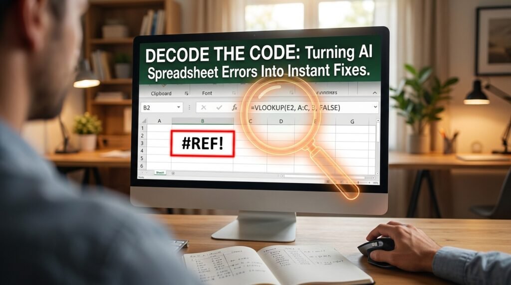
An AI-written formula that throws #VALUE! or #REF! the second you paste it usually failed for one of a few dull reasons, not because the logic was wrong. The error code tells you which one. Read the code first, isolate the piece that broke, then reprompt with the single detail the AI was missing, which is almost always your real column letters or your locale’s separator.
Read the error code before anything else
The code is a diagnosis, not just a complaint.
Each error points at a specific kind of failure, and Excel’s own error-checking reference lists what each one means. Match yours to the table below and you’ve already cut the problem in half.
Error | What it means | Common AI cause |
#REF! | A reference points nowhere | It guessed a column or row your sheet doesn’t have |
#VALUE! | Wrong type of value | Math on text, or a date stored as text |
#NAME? | Unknown name or function | A function from another app or locale, or a typo |
#DIV/0! | Division by zero or a blank | No guard for an empty denominator |
#N/A | A lookup found nothing | Exact-match lookup on values that don’t quite match |
#SPILL! | An array can’t expand | Cells in the spill range aren’t empty |
#NUM! | An invalid number | An impossible argument, like the root of a negative |
Most people skip this step and start rewriting the formula at random. The code already named the cause; you just have to read it.
One caution before you act: a cell can show an error that was really caused by a different cell it depends on. If the formula itself looks right, check the cells it points at before rewriting anything. The visible error isn’t always sitting where the actual problem lives.
The debugging decision tree
When the code alone doesn’t crack it, walk this in order.
Figure 1. From error code to cause to fix FORMULA ERRORS ON PASTE │ ▼ Is it #NAME? ──yes─► function name or separator wrong │ (check locale: comma vs semicolon) no ▼ Is it #REF! ──yes─► it used columns you don’t have │ (give it your real headers, re-ask) no ▼ Is it #VALUE! ──yes─► text where a number belongs │ (look for numbers-as-text, spaces) no ▼ Is it #N/A ──yes─► lookup keys don’t match │ (TRIM the keys; exact vs approx) no ▼ Still stuck? ──────► isolate: rebuild the formula one function at a time until it breaks |
Isolate the broken piece
A nested formula is several formulas wearing a trench coat.
When the cause isn’t obvious, take the formula apart. Copy an inner function into a spare cell and see what it returns on its own. In Excel, select a sub-expression inside the formula bar and press F9 to watch that piece evaluate; in Google Sheets, the hover tooltip and a few helper cells do the same job. Build outward from the part that works until you reach the part that doesn’t. The error is always at the seam between them.
Numbers stored as text: the quiet #VALUE!
This sits behind most #VALUE! errors people can’t explain.
A number that arrived from an export or a copy-paste is often text that merely looks like a number, and math on text fails. The tells are easy once you know them: the value hugs the left side of the cell instead of the right, Excel may flag it with a small green triangle, and ISNUMBER() returns FALSE. Two fixes cover most cases. Multiply the cell by 1 or wrap it in VALUE() to coerce it into a real number, and use Text to Columns to re-parse a whole column at once. A single trailing space is enough to cause this, so run TRIM first whenever you’re unsure.
When a lookup keeps returning #N/A
#N/A means the lookup searched and found nothing that matched.
With AI-written lookups, the match usually fails for a reason that has nothing to do with the formula. The keys don’t truly match: one side carries a trailing space, or one is the number 1004 while the other is the text ‘1004’, and those never line up. Exact-match lookups are unforgiving about both. Before you rewrite anything, TRIM both columns and confirm they hold the same data type, then decide whether you want an exact match or the approximate kind. Nine times in ten, #N/A is a data-matching problem wearing a formula’s clothes.
#REF! that shows up long after the formula was fine
This is the one error that can appear days after you wrote the formula.
When the AI builds a formula against specific cells and you later delete a column or row it pointed at, the reference has nowhere to land, and #REF! takes its place. The formula didn’t change; the ground under it did. You can rebuild the broken reference, but the larger lesson is that formulas pointing at fixed addresses are fragile. Asking the AI to reference whole columns or a named range, rather than A2:A50, makes a formula survive edits that would otherwise snap it.
The locale trap nobody warns you about

This one fools people who did everything right.
AI tools usually return formulas with comma separators, like =IF(A1>0, “yes”, “no”). In many regional settings, though, Excel and Sheets expect semicolons: =IF(A1>0; “yes”; “no”). A formula that is otherwise perfect throws a parse error or #NAME? purely because of that one character. The same regions often use a decimal comma instead of a point, which breaks numbers too. Tell the AI your locale up front, or swap the commas for semicolons by hand before you blame the logic.
Reprompt so it stops happening
The cure for guessed formulas is to remove the guessing.
Give the model the facts it was inventing: your exact headers and a sample row, which app and version you’re in, your locale separator, and what should happen when there’s no match. A prompt with those four things rarely errors on paste.
A prompt that removes every guess Write a formula for Google Sheets (US locale, commas). My data: A: Date (real dates) B: Region (text) C: Sales (number) Data starts in row 2 and runs to row 500.
Goal: total Sales where Region = “West” and the Date falls in 2026. If nothing matches, return 0, not an error.
Give me one formula to paste into E2, plus one line on how it works. |
This works because there’s nothing left to invent. The model can’t reach for a wrong column letter, a missing separator, or an unguarded divide, because you’ve already told it the answer to each.
Ask for formulas you can maintain
A formula you can’t read is a problem you’re saving for later.
AI tools love to hand back one enormous nested formula, because it’s compact, and compact is the opposite of maintainable. When the data shifts next month and it breaks, you’ll be debugging a wall of brackets you never understood in the first place. Ask differently. Tell the model to split the logic across a few helper columns, or to use named steps with LET so each part carries a label, and to add one line explaining what each piece does. The result runs a little longer and is far easier to fix. For anything you’ll reuse, readable beats clever.
A real debug, start to finish

Here’s the whole loop on a single broken formula.
Say the AI gave you =VLOOKUP(E2, A:C, 3, FALSE) and it returns #N/A. You read the code: a lookup found nothing. You isolate it by checking E2 against column A by eye, and the two look identical. So you test =E2=A5 in a spare cell, and it returns FALSE, which shouldn’t happen. That points at a hidden difference, so you try =TRIM(E2)=TRIM(A5), and now it reads TRUE. The culprit was a trailing space in the source data. No new formula was needed; cleaning the key with TRIM made the original lookup work. Reprompting would only have produced another VLOOKUP that failed the same way, because the formula was never the problem.
Questions people actually ask
It works in the AI’s example but not in my sheet. Why?
It built the example on placeholder ranges like A1:A10 that don’t line up with your data. Replace them with your real ranges, or better, give the model your headers and starting row up front so it never uses placeholders.
It says the function doesn’t exist.
That’s #NAME?, and it has three usual causes: a simple typo, a function that only exists in a different app or locale, or a newer function your version doesn’t include. Ask the model for an alternative that works in your specific app and version, and name them.
Should I trust a long nested formula it handed me?
Only once you can read it. Ask the model to explain each part in plain words, or have it split the logic into a couple of helper columns. A formula you can’t debug today is an error you can’t fix next month.
Why #SPILL! on a formula that worked yesterday?
A dynamic array needs empty cells to expand into, and something is now sitting in that range. Clear the cells below or beside the formula and the spill returns. Nothing is wrong with the formula itself.
Can I paste the error back and ask the AI to fix it?
You can, and it sometimes works, but only if you also paste what the AI can’t see: your real headers, a sample row, your app and locale, and what the formula is supposed to do. The error code alone doesn’t tell the model whether a column exists or whether a value is secretly text. Give it the same context you’d give a coworker, and the second attempt usually lands.
Read, isolate, reprompt
When the next AI formula errors out, don’t fire off a fresh request and hope. Read the error code to name the cause, isolate the failing sub-formula in a spare cell to confirm it, then reprompt with your real headers, your app, and your locale. Most syntax errors die at the first step, the moment you actually listen to what the code is telling you.

Hi I’m Muzammil Haqani. I’m a content creator and AI expert with 3+ years of experience exploring and writing about artificial intelligence and technology. Through this blog, I share tutorials, insights, and practical guides to help readers understand and use AI tools effectively in their everyday lives.